Wealth significantly influences how workers transition between jobs and employment states. When workers are unemployed, wealth may help them maintain their usual consumption levels and be more selective in their job search. Wealth may also encourage workers with a greater financial cushion to take potentially risky but high-paying jobs. However, wealth is often missing from standard labor market datasets. To fill this gap, recent work has turned to alternative data sources such the Survey of Income and Program Participation (SIPP) to document worker flows by wealth.
Yusuf Mercan and Jalen Nichols use data from the SIPP to study how household wealth—both in level and composition—shapes worker flows in the United States across a broader set of worker demographics. They find that workers in wealthier households tend to have lower job separation rates, modestly higher job-finding rates, and fewer job switches than workers in lower-wealth households. Liquid wealth has a stronger effect on job search behavior than illiquid wealth. Overall, their results suggest that individuals with higher and more liquid wealth tend to hold more stable jobs, and that lower-wealth workers may engage in more frequent job searching.
Article Citation
Mercan, Yusuf, and Jalen Nichols. 2025. "Understanding the Role of Wealth in Worker Flows." Federal Reserve Bank of Kansas City, Economic Review, vol. 110, no. 8. Available at External Linkhttps://doi.org/10.18651/ER/v110n8MercanNichols
Introduction
Wealth plays an important role in shaping how workers move between jobs and employment states. For example, when workers become unemployed, wealth may help them maintain their usual consumption levels and be more selective in their job search, reducing the urgency of accepting low-quality employment (Gruber 1997; Herkenhoff, Phillips, and Cohen-Cole 2024). Wealth may also affect how quickly workers climb the job ladder once employed, by encouraging workers with a greater financial cushion to take potentially risky but high-paying jobs (Clymo and others 2025).
Despite its role in shaping worker flows, wealth is often missing from standard labor market datasets, such as the Current Population Survey (CPS). This absence makes it infeasible to gauge the relationship between wealth and worker flows along a rich set of worker characteristics such as worker age, or type of wealth (liquid or illiquid). To fill this gap, recent work has turned to alternative data sources such the Survey of Income and Program Participation (SIPP) to document worker flows by wealth. For example, Krusell and others (2017) use the SIPP to focus on total net worth (including both liquid and illiquid assets), and Birinci and See (2023) measure how worker flows depend on net liquid wealth but do not study employer-to-employer transitions.
In this article, we also use data from the SIPP to complement this growing body of research and study how household wealth—both in level and composition—shapes worker flows in the United States across a broader set of worker demographics. Our findings are in line with previous studies. Namely, we find that workers in wealthier households tend to have lower job separation rates, modestly higher job finding rates, and fewer job switches than workers in lower-wealth households. However, we also find that not all wealth influences labor market behavior in the same way. Liquid wealth—that is, assets that can be readily accessed, such as checking accounts—has a stronger effect on job search behavior than illiquid wealth such as housing equity or retirement savings. Overall, our results suggest that individuals with higher and more liquid wealth tend to hold more stable jobs, and that lower-wealth workers may engage in more frequent job searching, possibly due to job instability or the pursuit of better opportunities.
Section I illustrates the importance of studying worker flows for a full understanding of the labor market. Section II describes our data and measurement approach. Section III presents empirical patterns in worker flows by wealth and examines how wealth liquidity shapes these transitions.
I. Importance of Flows in Shaping Workers’ Labor Market Experiences
Understanding how workers move between employment states and jobs is crucial for getting a comprehensive picture of the labor market. Standard labor market indicators such as the unemployment rate provide only a snapshot of labor market conditions, masking the underlying movements of workers. The pace at which unemployed workers find a job, for example, determines how quickly an economy can recover from downturns. When the job-finding rate is high, a negative shock that leads to a spike in unemployment will dissipate quickly. However, in a more stagnant economy where unemployed workers find jobs more slowly, the same negative shock will leave the unemployment rate higher for longer. Similarly, the speed at which workers switch jobs while employed is a crucial factor determining wage growth, aggregate productivity, and inflation, among other macroeconomic outcomes. When workers switch jobs, they typically move to higher-productivity firms at higher pay, which are important factors that determine the productive capacity of an economy and aggregate consumption (Haltiwanger, Hyatt, and McEntarfer 2018; Davis and Haltiwanger 2014; Topel and Ward 1992; Ozkan, Song, and Karahan 2023)._
To capture these dimensions of the labor market, we study three types of worker flows on a monthly basis: the unemployment-to-employment (UE) transition rate, which measures the share of unemployed workers who find a job; the employment-to-unemployment (EU) transition rate, which measures the share of employed workers who lose their job; and the employer-to-employer (EE) transition rate, which measures the share of employed workers who switch to a different job._
Chart 1 plots these rates over time and illustrates two key observations._ First, the U.S. labor market is highly dynamic. The green line shows that roughly 25 percent of unemployed workers find jobs each month, suggesting that, on average, a worker spends four months unemployed before finding a job. The blue line shows that, on average, 1.5 percent of employed workers transition into unemployment each month, suggesting that an average worker spends about 5.5 years in employment before becoming unemployed. And the purple line shows that around 2 percent of employed workers switch jobs each month. Relative to other advanced economies, U.S. labor market flow rates are the highest, indicating a dynamic labor market (Elsby, Hobijn, and Şahin and 2013; Borowczyk-Martins 2025).
Chart 1: Worker Flows in the United States
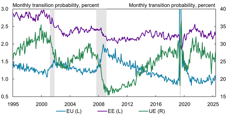
Notes: Chart plots the monthly employment-to-unemployment (EU), employer-to-employer (EE) and employment-to-unemployment (EU) transition probabilities in the United States. Gray bars indicate National Bureau of Economic Research (NBER)-defined recessions.
Sources: U.S. Census Bureau and U.S. Bureau of Labor Statistics (accessed via Federal Reserve Bank of St. Louis, FRED), Fujita, Moscarini, and Postel-Vinay (2024), NBER, and authors’ calculations.
Second, worker flows in the United States show a strong relationship with the business cycle. Chart 1 shows that the UE and EE rates (green and purple lines, respectively) are procyclical—that is, they rise during expansions and fall in recessions. Intuitively, workers find it easier to find a new job during economic expansions. In contrast, the EU rate (blue line) is countercyclical, increasing sharply during economic downturns and declining gradually during recoveries. This relationship is similarly intuitive, implying that the likelihood of a job loss is higher during recessionary episodes.
While these aggregate worker flow rates help illustrate the underlying worker movements in the labor market, they may mask differences across different types of workers. The U.S. labor market consists of workers of various ages, wealth and income levels, and educational backgrounds, who are employed in different industries and occupations. Each of these factors may shape how workers move through employment states, influencing both aggregate macroeconomic outcomes in the United States as well as workers’ individual labor market experiences.
II. Measuring Worker Flows with the SIPP
Worker demographics are likely to play a role in determining the pace of their transitions between jobs and employment states in the labor market. Wealth in particular may have a strong influence on worker flows. These flows, in turn, determine how long a worker spends in unemployment versus employment, as well as the duration of their employment relationship with a given firm. However, assessing how worker flows vary by household wealth can be challenging, as many common labor market datasets such as the CPS, the standard reference source, do not include measures of household wealth. We therefore use the U.S. Census Bureau’s Survey of Income and Program Participation (SIPP) to allow for a granular empirical analysis based on household wealth.
The SIPP is a longitudinal survey composed of multiple panels, each spanning several years. Its structure enables us to track workers’ employment status over time and to construct measures of household wealth. In the 1996–2008 panels, respondents are interviewed three times per year about the preceding four months; in the 2014–23 panels, respondents are interviewed once a year about the prior year. We combine data from all available panels from 1996 to 2023, covering the period from December 1995 to December 2022, with time gaps where adjacent panels do not overlap. Further details on sample selection and variable construction are available in Appendix B.
Measuring gross worker flows
The SIPP reports the monthly employment status for each respondent, which allows us to construct transition rates between different labor market states. Namely, we define the UE rate as the share of unemployed workers who find jobs between two months and the EU rate as the share of employed workers who lose a job from one month to the next. We further define the EE transition rate as the share of employed workers who change employers from one month to the next. To identify such job switches, we track each worker’s employer identification number for their main job. We record a worker as having made an EE switch whenever this ID changes._
Measuring wealth
In addition to employment status, the SIPP also collects detailed information on household assets and liabilities. Respondents report asset and debt positions across a variety of categories. We define a household’s wealth as its total net worth (assets net of liabilities). In our analysis, we further distinguish between liquid and illiquid wealth. Liquid wealth includes interest-earning bank accounts, stocks, and mutual funds net of unsecured debt (such as credit card balances). Illiquid wealth includes equity in real estate, businesses, vehicles, and retirement accounts. This categorization allows us to examine not only the overall level of household wealth, but also its composition._
III. Worker Flows by Wealth
We study the three worker transition rates by quintile of wealth using the SIPP. We present results by quintile for both total net worth and liquid wealth. Breakdowns for various age, education, industry, and occupation categories by wealth that emerge from our analysis are available in tables in Appendix C.
Unemployment-to-employment transitions
Overall, job-finding rates increase modestly with wealth. The green bars in Chart 2 present UE transition rates by different net worth quintiles._ Workers in the bottom wealth quintile find jobs at a rate of 14 percent per month, while those in the top two quintiles find jobs at rates closer to 17 percent.
Chart 2: Average Worker Flows by Total Net Worth
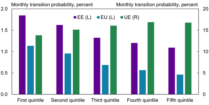
Sources: U.S. Census Bureau and authors’ calculations.
However, this relationship with wealth varies based on age and education level (detailed results across demographic groups are available in Appendix C). Looking across age groups, the job-finding rates increase with wealth for younger workers (age 15–24) but are relatively flat for prime-age workers (age 25–54). By contrast, job-finding rates by occupation and industry across wealth groups show no clear patterns._ In short, the UE rate rises only slightly with household wealth and exhibits considerable variation across demographic groups. This suggests that wealth may not substantially influence how unemployed workers search for jobs.
Employment-to-unemployment transitions
Wealth effects are much stronger for EU transition rates, shown in the blue bars in Chart 2. Workers in higher-wealth households are far less likely to lose their jobs. The monthly job loss rate declines consistently as wealth increases, from 1.14 percent in the bottom quintile to just 0.46 percent in the top quintile. This negative relationship between wealth and job loss is robust across all demographic groups.
While younger, less-educated workers and those in manual occupations face higher unemployment risk on average, household wealth provides a significant buffer within each of these high-risk groups (see Appendix C, Table 2). In sum, although job-finding rates rise only modestly with wealth, job-losing rates decline more dramatically and consistently with wealth. In other words, higher wealth is strongly associated with more stable employment: higher-wealth workers are more likely to be in well-matched and secure jobs, and lower-wealth individuals are more likely to lose their jobs once employed, hampering their wealth accumulation.
Employer-to-employer transitions
Job switching declines markedly with wealth, as seen in the purple EE transition rate bars in Chart 2—similar to the patterns observed in EU rates by wealth—suggesting higher-wealth workers are more likely to be in well-matched, secure, and better-paying jobs. In contrast, workers in lower-wealth households appear more likely to switch jobs in pursuit of better opportunities.
Interestingly, this pattern does not hold for younger workers: Their job switching rates are relatively flat across the wealth distribution, likely reflecting broader career exploration early in life (see Appendix C, Table 3). A similar pattern emerges among workers with lower education levels. Overall, job mobility declines with wealth, and younger, less-educated, or lower-skilled workers switch jobs more frequently—consistent with lower-quality or short-term jobs.
Does the nature of wealth matter for labor market flows?
Our results thus far show substantial variation in worker flows between employment and unemployment—and across employers—by household wealth. Although individuals in high-wealth households tend to experience more stable employment, as reflected in lower EU and EE rates, the UE rate shows only a modest positive correlation with wealth.
However, these results are based on household net worth—a combination of liquid assets (such as bank accounts) and illiquid assets (such as home equity). The relationships documented thus far may vary further based on the composition of wealth. Not all types of wealth are equally accessible to individuals in times of need. Liquid assets may support longer or more selective job search in unemployment, while illiquid wealth is harder to draw upon in the short run. These considerations may influence workers’ labor market behavior.
To account for this possibility, Chart 3 shows worker flows by liquid and illiquid wealth quintiles. Overall, the chart reveals two key patterns. First, patterns based on illiquid wealth (Panel B) closely resemble those for net worth—unsurprising, given that illiquid assets dominate household balance sheets. Second, the UE rate behaves differently conditional on liquid wealth (Panel A). In particular, the UE rate is relatively high among households in the bottom quintile of liquid wealth—higher than among the middle 60 percent—potentially indicating increased search intensity among liquidity-constrained workers.
Chart 3: Average Worker Flows by Liquid and Illiquid Wealth
Panel A: Liquid Wealth
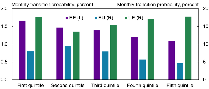
Panel B: Illiquid Wealth
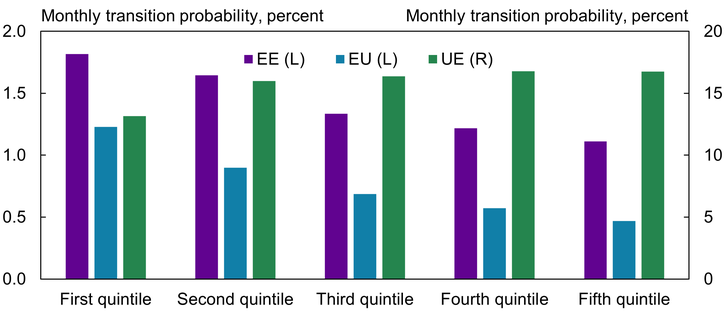
Sources: U.S. Census Bureau and authors’ calculations.
In summary, worker flows by wealth type follow similar patterns as those for net worth, except for the job-finding rate. Having low levels of liquid wealth is associated with a higher UE rate relative to the middle of the wealth distribution, suggesting an important role for government policies such as unemployment insurance that provides liquidity to low-liquidity individuals.
Conclusion
Household wealth plays a substantial role in shaping labor market dynamics in the United States. Using data from the SIPP, we document that workers in wealthier households face lower job loss rates and switch jobs less frequently. Although workers in wealthier households also have higher job-finding rates, this effect is more modest. We also find that the composition of this wealth matters. Workers with lower liquid wealth—assets that are readily accessible—have a higher job-finding rate than workers with a similar level of illiquid wealth.
Our results suggest that wealth, particularly in liquid form, is a key determinant of labor market mobility. Workers with limited financial buffers may be compelled to accept job offers more quickly, potentially leading to poorer job matches. In contrast, those with greater liquidity can afford longer and more selective searches, enabling better matches that may enhance both individual well-being and aggregate labor market outcomes.
These findings have several policy implications. Programs that enhance financial resilience—such as emergency savings incentives, targeted cash transfers, or expanded access to unemployment insurance—may reduce labor market instability among low-wealth households. Furthermore, policies that support the accumulation of not just wealth, but accessible and flexible forms of wealth, could improve the efficiency of labor market outcomes. Finally, policymakers might consider the labor market consequences of the baby boom generation retiring and transferring their wealth to prime-age workers. This wealth transfer may result in a less dynamic U.S. labor market, slowing down the speed of labor market adjustment to adverse economic shocks.
Appendix A: Deriving the Half-Life of Unemployment
Two economies with identical unemployment rates but different underlying worker flows may exhibit starkly different responses to economic shocks. To illustrate this point, we consider a simplified labor market in which workers are either employed or unemployed, and the total labor force is normalized to one. For simplicity, we ignore transitions within employment (that is, job-to-job flows).
Suppose a fraction ft of unemployed workers find jobs and a fraction δt of employed workers lose their jobs in each month t. The unemployment rate, ut, then evolves according to the following equation:
ut+1 − ut = −ftut + δt(1 − ut).
The first term on the right-hand side captures unemployed workers finding jobs and exiting unemployment. The second term captures employed workers losing their jobs and entering unemployment. In a steady state—when aggregate outcomes remain constant over time—the unemployment rate is a constant ū. This allows us to solve for the steady-state unemployment rate as a function of worker flows as ū = δ / (δ + f). This steady-state expression reveals that the unemployment rate depends directly on the relative magnitudes of job separation and job finding probabilities in the labor market.
For context, we consider the U.S. labor market between 1990 and 2007. In this period, the average monthly job finding rate was f = 0.27 and the average job separation rate was δ = 0.014, which imply a steady-state unemployment rate of ū = 0.014 / (0.014 + 0.27) ≈ 5 percent. This estimate closely matches the actual U.S. unemployment rate of 5.4 percent over the same period._
We also consider an alternative economy where the labor market is “frozen” and both job-finding and job-separation probabilities are half as large—specifically, f = 0.135 and δ = 0.007. In this economy, workers are less likely to lose their jobs but have a harder time finding a job once unemployed. Crucially, the steady-state unemployment rate ū = 0.007 / (0.007 + 0.135) ≈ 5 percent remains the same as before, as both the numerator and denominator change proportionally. However, the two economies react very differently to shocks.
To see this point, we consider a one-time temporary rise in the job separation probability δ, such as might occur during a recession. The half-life (defined in the subsection below) of such a shock is drastically different between the two economies. The time it takes for the unemployment rate to recover to half its initially elevated level following this adverse shock is about two months in the first, more fluid economy, whereas it is 4.5 half months in the second, more stagnant economy.
This example highlights that two economies can have the same unemployment rate yet differ dramatically in labor market dynamics. The pace of flows between employment and unemployment is a key determinant of how quickly the economy adjusts to shocks. More broadly, understanding worker flow patterns—including employer-to-employer transitions—is crucial for a complete characterization of the labor market.
The half-life of employment
We assume constant job-finding and job-separation rates. Under this assumption, the law of motion for the unemployment rate ut is given by:
ut+1 = (1 − f)ut + δ(1 − ut).
Recalling the definition of the steady-state unemployment rate ū = δ / (δ + f), one can express the unemployment law of motion as:
ut+1 − ū = (1 − f − δ)(ut − ū).
Iterating forward from t = 0, we obtain:
ut − ū = (1 − f − δ)t(u0 − ū).
The half-life of unemployment is defined as the time t = t1/2 at which the deviation from the steady state is halved:
(ut − ū)/(u0 − ū) = 0.5 = (1 − f − δ)t.
Solving for t yields:
t1/2 = (log(0.5))/(log(1 − f − δ)).
This expression provides a simple closed-form formula for the half-life of unemployment under constant flow rates following a one-time transitory increase in the job separation rate.
Appendix B: Further Details on Measurement in the SIPP
We define the unemployment-to-employment and employment-to-unemployment rates in month t as:
UEt = (Ut → Et+1) / Ut and EUt = (Et → Ut+1) / Et.
Here, Et and Ut denote the number of employed and unemployed workers in month t, respectively. Et → Ut+1 is the number of employed workers in month t who are observed to be unemployed in month t + 1. Similarly, Ut → Et+1 is the number of unemployed workers in month t who have a job in month t + 1. Analogously, we define the employer-to-employer (EE) transition rate in month t as the share of workers who are employed in two consecutive months, but who have changed employers.
We restrict our sample to households with available net worth information and to individuals between the ages of 15 and 65. Census industry and occupation codes undergo several revisions between 1995 and 2023, the period covered by our sample. To harmonize these classifications over time, we follow the concordance approach in Acemoglu and Autor (2011), using a consistent set of 10 major industry categories and four broad occupation groups.
Appendix C: Detailed Worker Flows by Demographic Groups and Net Worth Quintiles
Table 1: UE Rates by Demographic Groups and Net Worth Quintiles
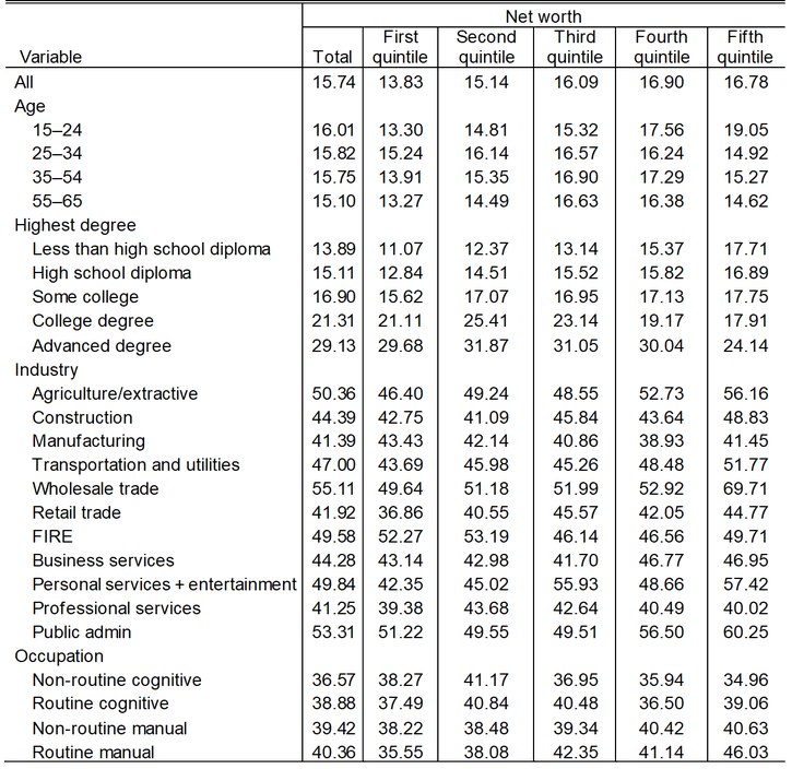
Notes: Table reports the monthly unemployment-to-employment (UE) transition probability in the United States for various demographic groups by their wealth holdings. All values are in percentage points.
Sources: U.S. Census Bureau and authors’ calculations.
Table 2: EU Rates by Demographic Groups and Net Worth Quintiles
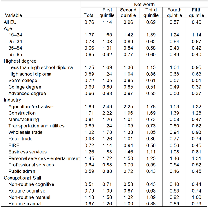
Notes: Table reports the monthly employment-to-unemployment (EU) transition probability in the United States for various demographic groups by their wealth holdings. All values are in percentage points.
Sources: U.S. Census Bureau and authors’ calculations.
Table 3: EE Rates by Demographic Groups and Net Worth Quintiles
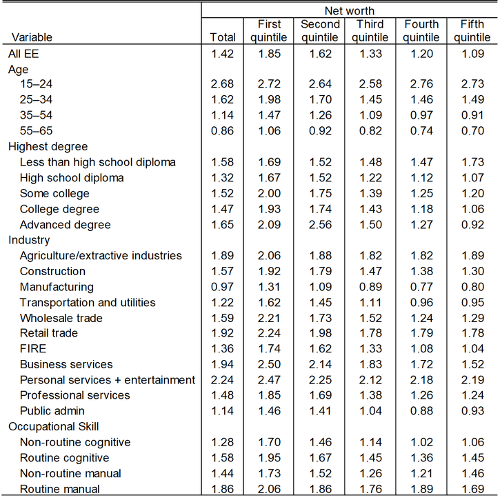
Notes: Table reports the monthly employer-to-employer (EE) transition probability in the United States for various demographic groups by their wealth holdings. All values are in percentage points.
Sources: U.S. Census Bureau and authors’ calculations.
Endnotes
-
1 Labor market flows also have implications for macroeconomic policy. For example, Moscarini and Postel-Vinay (2023) and Birinci and others (2025) study how the frequency of job switching shapes inflationary pressures in an economy and what this implies for the conduct of monetary policy.
-
2 As is standard in prior research, we use the term “rate” to refer to these shares. More precisely, these are discrete-time transition probabilities. When constructing aggregate moments from the microdata, we apply the person-level sampling weights provided by the SIPP. We abstract from other relevant labor market margins, such as flows into and out of the labor force. Although flows into and out of the labor force are not negligible in size (for example, around 2.8 percent of the employed exit the labor force each month), this simplification allows us to narrow our analysis. More broadly, other important worker flow margins shape the U.S. economy that we do not study here. For example, in the 2025 Jackson Hole Economic Policy Symposium on “Labor Markets in Transition—Demographics, Productivity and Macroeconomic Policy,” Foschi and others (2025) presented work on the changing patterns in inter-state labor mobility in the United States and what they imply for place-based policies versus removing barriers to migration between U.S. states.
-
3 For details on how to measure worker flows in the CPS, see Mercan, Schoefer, and Sedláček (2024).
-
4 The SIPP allows respondents to report multiple jobs held in each month. If a worker reports more than one job, we define their main job as the one with the most hours worked per week.
-
5 Researchers have documented that flow rates in the CPS and SIPP differ in levels (Fujita, Nekarda, and Ramey 2007; Krusell and others 2017). Since our focus in this article is on cross-group differences rather than precise levels, we do not adjust for these discrepancies. For similar reasons, we do not adjust the transition rates constructed using the SIPP for other potential sources of bias, such as time aggregation or margin error.
-
6 Quintiles divide a population into five equally sized groups based on a variable—in this case, household net worth. For example, the first quintile represents the poorest 20 percent of the sample, the second quintile represents the next poorest 20 percent, and so on.
-
7 Job-finding probabilities by industry and occupation are significantly higher than the unconditional averages due to strong selection effects. The SIPP records the industry and occupation of unemployed workers based on their last held job. These individuals tend to be more attached to the labor force and are therefore more likely to find employment, resulting in higher measured UE rates.
-
8 A more precise steady-state approximation to the unemployment rate involves using continuous-time methods to correct for time aggregation bias. With this method, the average steady-state approximation becomes 5.4 percent, which closely matches the actual unemployment rate. See Shimer (2012) for details.
Article Citation
Mercan, Yusuf, and Jalen Nichols. 2025. "Understanding the Role of Wealth in Worker Flows." Federal Reserve Bank of Kansas City, Economic Review, vol. 110, no. 8. Available at External Linkhttps://doi.org/10.18651/ER/v110n8MercanNichols
Publication information: Vol. 110, no. 8
DOI: 10.18651/ER/v110n8MercanNichols
References
Acemoglu, Daron, and David Autor. 2011. “Chapter 12 - Skills, Tasks and Technologies: Implications for Employment and Earnings.” Handbook of Labor Economics, vol. 4, pt. B, pp. 1043–1171. Available at External Linkhttps://doi.org/10.1016/S0169-7218(11)02410-5
Birinci, Serdar, and Kurt See. 2023. “Labor Market Responses to Unemployment Insurance: The Role of Heterogeneity.” American Economic Journal: Macroeconomics, vol. 15, no. 3, pp. 388–430. Available at External Linkhttps://doi.org/10.1257/mac.20200057
Birinci, Serdar, Fatih Karahan, Yusuf Mercan, and Kurt See. 2025. “Labor Market Shocks and Monetary Policy.” Federal Reserve Bank of Kansas City, Research Working Paper no. 24-04, May. Available at External Linkhttps://doi.org/10.18651/RWP2024-04
Borowczyk-Martins, Daniel. 2025. “Employer-to-Employer Mobility and Wages in Europe and the United States.” IZA Discussion Paper no. 17719. Available at External Linkhttps://doi.org/10.2139/ssrn.5147080
Clymo, Alex, Piotr Denderski, Yusuf Mercan, and Benjamin Schoefer. 2025. “The Job Ladder, Unemployment Risk, and Incomplete Markets.” Working paper.
Davis, Steven J., and John Haltiwanger. 2014. “Labor Market Fluidity and Economic Performance.” National Bureau of Economic Research, working paper no. 20479, September Available at External Linkhttps://doi.org/10.3386/w20479
Elsby, Michael W. L., Bart Hobijn, and Ayşegül Şahin. 2013. “Unemployment Dynamics in the OECD.” Review of Economics and Statistics, vol. 95, no. 2, pp. 530–548. Available at External Linkhttps://doi.org/10.1162/REST_a_00277
Foschi, Andrea, Christopher L. House, Christian Proebsting, and Linda L. Tesar. 2025. “Interstate-State Labor Mobility and the U.S. Economy.” Working paper presented at the Federal Reserve Bank of Kansas City Economic Policy Symposium, Jackson Hole, WY, August 22.
Fujita, Shigeru, Giuseppe Moscarini, and Fabien Postel-Vinay. 2024. “Measuring Employer-to-Employer Reallocation.” American Economic Journal: Macroeconomics, vol. 16, no. 3, pp. 1–51. Available at External Linkhttps://doi.org/10.1257/mac.20210076
Fujita, Shigeru, Christopher J. Nekarda, and Garey Ramey. 2007. “The Cyclicality of Worker Flows: New Evidence from the Sipp.” Federal Reserve Bank of Philadelphia, working paper, February. Available at External Linkhttps://doi.org/10.21799/frbp.wp.2007.05
Gruber, Jonathan. 1997. “The Consumption Smoothing Benefits of Unemployment Insurance.” American Economic Review, vol. 87, no. 1, pp. 192–205.
Haltiwanger, John, Henry Hyatt, and Erika McEntarfer. 2018. “Who Moves Up the Job Ladder?” Journal of Labor Economics, vol. 36, no. S1, pp. 301–336. Available at External Linkhttps://doi.org/10.1086/694417
Herkenhoff, Kyle, Gordon Phillips, and Ethan Cohen-Cole. 2024. “How Credit Constraints Impact Job Finding Rates, Sorting, and Aggregate Output.” Review of Economic Studies, vol. 91, no. 5, pp. 2832–2877. Available at External Linkhttps://doi.org/10.1093/restud/rdad104
Krusell, Per, Toshihiko Mukoyama, Richard Rogerson, and Ayşegül Şahin. 2017. “Gross Worker Flows over the Business Cycle.” American Economic Review, vol. 107, no. 11, pp. 3447–3476. Available at External Linkhttps://doi.org/10.1257/aer.20121662
Mercan, Yusuf, Benjamin Schoefer, and Petr Sedláček. 2024. “A Congestion Theory of Unemployment Fluctuations.” American Economic Journal: Macroeconomics, vol. 16, no. 1, pp. 238–285. Available at External Linkhttps://doi.org/10.1257/mac.20210171
Moscarini, Giuseppe, and Fabien Postel-Vinay. 2023. “The Job Ladder: Inflation vs. Reallocation.” National Bureau of Economic Research, working paper no. 31466, July. Available at External Linkhttps://doi.org/10.3386/w31466
Ozkan, Serdar, Jae Song, and Fatih Karahan. 2023. “Anatomy of Lifetime Earnings Inequality: Heterogeneity in Job-Ladder Risk versus Human Capital.” Journal of Political Economy Macroeconomics, vol. 1, no. 3. Available at External Linkhttps://doi.org/10.1086/725790
Shimer, Robert. 2012. “Reassessing the Ins and Outs of Unemployment.” Review of Economic Dynamics, vol. 15, no. 2, pp. 127–148. Available at External Linkhttps://doi.org/10.1016/j.red.2012.02.001
Topel, Robert H., and Michael P. Ward. 1992. “Job Mobility and the Careers of Young Men.” Quarterly Journal of Economics, vol. 107, no. 2, pp. 439–479. Available at External Linkhttps://doi.org/10.2307/2118478
Yusuf Mercan is a senior economist at the Federal Reserve Bank of Kansas City. Jalen Nichols is a former research associate at the bank. The views expressed are those of the authors and do not necessarily reflect the positions of the Federal Reserve Bank of Kansas City or the Federal Reserve System.
Author