Since 2017, many state governments have seen solid growth in tax revenue collections. According to the Fiscal Survey of States produced by the National Association of State Budget Officers, state revenue collections grew by 7.0 percent on a nominal basis in fiscal year 2018, compared with 2.4 percent in fiscal 2017 and 1.8 percent in fiscal 2016. The strong gains in April tax collections led many states to end fiscal 2019 with revenue growth higher than estimated.
Recent changes in the federal tax code on personal income through the Tax Cuts and Jobs Act (TCJA) have contributed to the uptick in state revenues. The size of this uptick varies depending on how states choose to measure personal income. Different states may use federal tax income (FTI), federal adjusted gross income (AGI), or their own definition of income as a starting point for state income taxes._The majority of changes in the TCJA that broadened the tax base, such as eliminating personal exemptions and limiting itemized deductions, directly affected FTI but not AGI. Chart 1 shows that growth in tax revenues was similar across the three groups of states in fiscal 2017 and is expected to be similar once more in fiscal 2019. In fiscal 2018, however, states using FTI saw much stronger growth than other states, as they directly inherited most changes in the federal tax reform. States using AGI or their own income definitions would have needed to take legislative actions to conform with the federal tax code.
Chart 1: Growth of Personal Income Tax Revenue across States
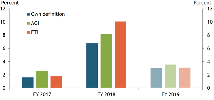
Notes: Growth rates for fiscal 2019 are estimates and likely to be revised higher due to strong gains in April tax collections. States are grouped according to the Federation of Tax Administrators and individual state statutes as in Auxier and Sammartino (2018).
Sources: National Association of State Budget Officers and authors’ calculations.
States have used the recent revenue windfall to build up their rainy day funds, reserves that help them manage budget shortfalls during economic downturns. Most states are required to maintain a balanced budget on operating expenditures and cannot carry a deficit from one fiscal year into the next._Therefore, state governments usually put aside more reserves during economic expansions and tap into their rainy day funds during economic downturns.
Chart 2 shows that states have built up rainy day funds at a much faster pace than before the Great Recession. From fiscal 2003 to 2007, GDP-weighted state revenue grew at an average annual rate of 7.3 percent. Over the same period, states raised their GDP-weighted average of rainy day funds (measured as a share of state expenditures) by only 0.44 percent. In fiscal 2018, state revenue grew at a slightly faster pace, but the increase in rainy day funds more than tripled to 1.52 percent. More generally, states have been putting a larger share of their revenue into rainy day funds since the Great Recession. From fiscal 2011 to 2018, state revenues grew at an average annual rate of less than 5 percent, while rainy day funds as a share of state expenditures grew by 0.63 percent. The larger buffers that state governments have built in recent years may help them mitigate expenditure cuts in the event of an economic downturn.
Chart 2: Growth of State Tax Revenue and Change in Rainy Day Funds Balance
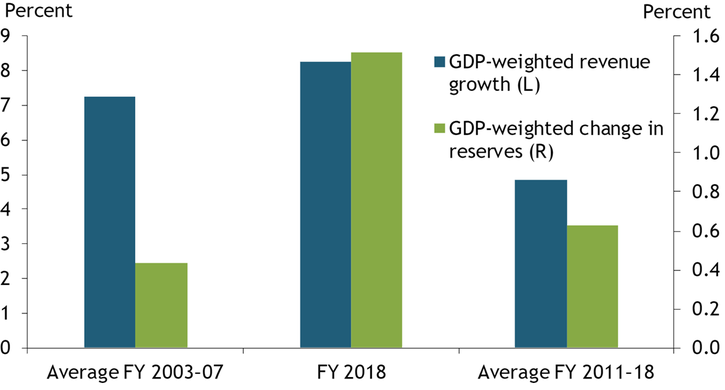
Note: For the GDP-weighted average measure, more weight is assigned to states with higher state GDP.
Sources: U.S. Census Bureau, PEW Charitable Trusts, and authors’ calculations.
The savings behavior of individual states also appears to have changed since the Great Recession. Before the recession, states with smaller rainy day fund balances did not appear to invest many resources in shoring up these funds. The horizontal axis in Chart 3 shows the size of states’ rainy day fund balances (as a share of state expenditures) in 2006, while the vertical axis shows how these balances grew from 2006 to 2007. Comparing the two axes shows that states that had relatively larger rainy day funds in fiscal 2006, such as Nebraska and North Dakota, saved more than states with smaller funds in fiscal 2007.
Chart 3: Rainy Day Fund Balance in Fiscal 2006 and Change in Balance from Fiscal 2006 to Fiscal 2007
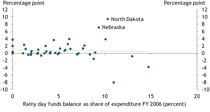
Note: Alaska and Wyoming are excluded from this plot, as the balances of their rainy day funds are substantially larger than the median.
Sources: National Association of State Budget Officers and authors’ calculations.
In contrast, states with smaller buffers that are therefore more vulnerable to budget shortfalls have been saving more in their rainy day funds in recent years. Chart 4 shows that in fiscal 2017, the balances of rainy day funds fell within a broad range across states: four states had no reserves, and Texas had a balance sufficient to cover 19 percent of state expenditures. However, by fiscal 2018, states with smaller or no rainy day funds, such as New Mexico, Connecticut, and Oklahoma, had raised their rainy day funds at a much faster pace than most states. The deep expenditure cuts that states had to take during the Great Recession may have prompted states with smaller buffers to shore up their rainy day funds.
Chart 4: Rainy Day Fund Balance in Fiscal 2017 and Change in Balance from Fiscal 2017 to Fiscal 2018
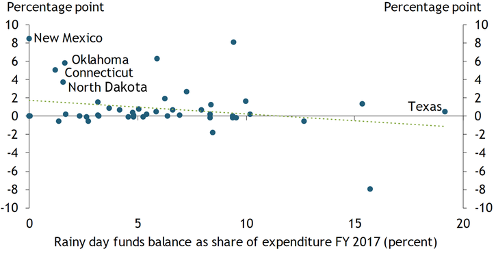
Note: Alaska and Wyoming are excluded from this plot, as the balances of their rainy day funds are substantially larger than the median.
Sources: National Association of State Budget Officers and authors’ calculations.
This analysis yields two takeaways. First, changes in the federal tax code have played an important role in the recent surge in state revenues, as states that more closely align with the federal tax code have seen larger increases in their revenues. Second, states have used recent revenue windfalls to build up rainy day funds at a faster pace than before the Great Recession. The stronger buffers that they have built may help state governments mitigate the scope of budget cuts in the event of an economic downturn.
Endnotes
-
1 AGI is a taxpayer’s gross income after “above-the-line” adjustments, such as deductions for individual retirement account contributions, student loan interest, and moving expenses. The FTI is the AGI minus “below-the-line” items, including personal exemptions or standard or itemized deductions.
-
2 Most state governments have separate operating and capital budgets, and they can borrow to support capital expenditures.
Reference
Auxier, Richard, and Frank Sammartino. 2018. External LinkThe Tax Debate Moves to the States: The Tax Cuts and Jobs Act Creates Many Questions for States that Link to Federal Income Tax Rules.” Tax Policy Center, January 23.
Huixin Bi is a research and policy officer at the Federal Reserve Bank of Kansas City. Jaeheung Bae is a research associate at the bank. The views expressed are those of the authors and do not necessarily reflect the positions of the Federal Reserve Bank of Kansas City or the Federal Reserve System.
Author